
Kо̄manawa-Base#
- Author:
Matt Dumont
- copyright:
2024, Kо̄manawa Solutions Ltd.
- Version:
v2.4.0
- Date:
Feb 23, 2026
What is BASE?#
The Bayesian Approach to Source Estimation (BASE) is a method to conduct a Bayesian analysis to constrain a prior of the source concentration of a given groundwater receptor (e.g. well, spring fed stream, etc.) with the measured concentration at the receptor and an inferred age distribution (e.g. via tritium sampling).
The assumptions of BASE.#
BASE makes the following assumptions:
The source concentration varies smoothly with time.
That any variation in receptor concentration that cannot be explained by the source concentration parametrisation is due to unexplained variance e.g. measurement error, model error, etc.
That the True source concentration exists within the prior distribution defined by the user.
That the ground water age distribution is known and does not vary with time, recharge rates, etc.
How to Cite#
Please cite this via our paper: Bayesian inference to predict past and future nitrate concentrations (https://doi.org/10.1016/j.jconhyd.2026.104902)
Bibtex entry:
@article{DUMONT2026104902,
title = {Bayesian inference to predict past and future nitrate concentrations},
journal = {Journal of Contaminant Hydrology},
pages = {104902},
year = {2026},
issn = {0169-7722},
doi = {https://doi.org/10.1016/j.jconhyd.2026.104902},
url = {https://www.sciencedirect.com/science/article/pii/S016977222600063X},
author = {Matt Dumont and Connor Cleary and Richard McDowell},
keywords = {Lag, Nitrate, Leaching, Groundwater, Lumped-parameter-model, Land-management},
}
Installation#
To install BASE, you can use pip:
See known issues in dependencies section below regarding numpy 2.4.
pip install komanawa-BASE
Alternatively, you can install the latest version from the GitHub repository:
pip install git+https://github.com/Komanawa/komanawa-BASE.git
Dependencies#
BASE requires the following packages:
numpy
pandas
matplotlib
scipy
psutil
pytables (for hdf support)
openpyxl (for excel support)
komanawa-gw-age-tools (for gw age distribution inference)
pydream (for DREAMzs solver)
Known issues#
Numpy 2.4 breaks the current implementation of pydream, which is a dependency of BASE. For now, we recommend using an earlier version of numpy (2.3 or earlier) to avoid this issue.
Resource Requirements#
BASE is a relatively lightweight model, but it is a Bayesian model and thus has higher computational requirements than something like a simple regression model. To provide some clarity on the resource requirements, we have included a runtime_memtest.py script which has functions that can be imported to run time and memory tests or it can be called directly from the command line to run a test on the current machine.
When we ran the tests on a local machine (AMD Ryzen 5 7600X 6-Core Processor) we found the run time for 4 chains and 25000 iterations with 1 year inflections (39 inflection points) to be c. 117 seconds. The memory usage was c. 150 MiB.
Usage#
A full worked example(s) of how to use BASE is provided in the following jupyter notebook:
Otherwise detailed documentation is provided in the code documentation for the relevant classes and methods. The main classes and modules are:
BaseSampledParam: Schema for a prior parameter which allows serialisation.
BASESolver: The main class, constrain a prior of the source concentration with the observed data at a single site and an inferred binary exponential piston flow lumped parameter age model.
MultiSiteBASESolver: Constrain a common prior source concentration with the observed data at multiple sites and an inferred binary exponential piston flow lumped parameter age model (unique age distribution for each site).
MultiSiteDilutionBASESolver: Constrain a common prior source concentration with the observed data at multiple sites and an inferred binary exponential piston flow lumped parameter age model (unique age distribution for each site) allowing for a scalar dilution factor to be applied for each site.
generators: Access to generator to support prior development.
Interpolation options#
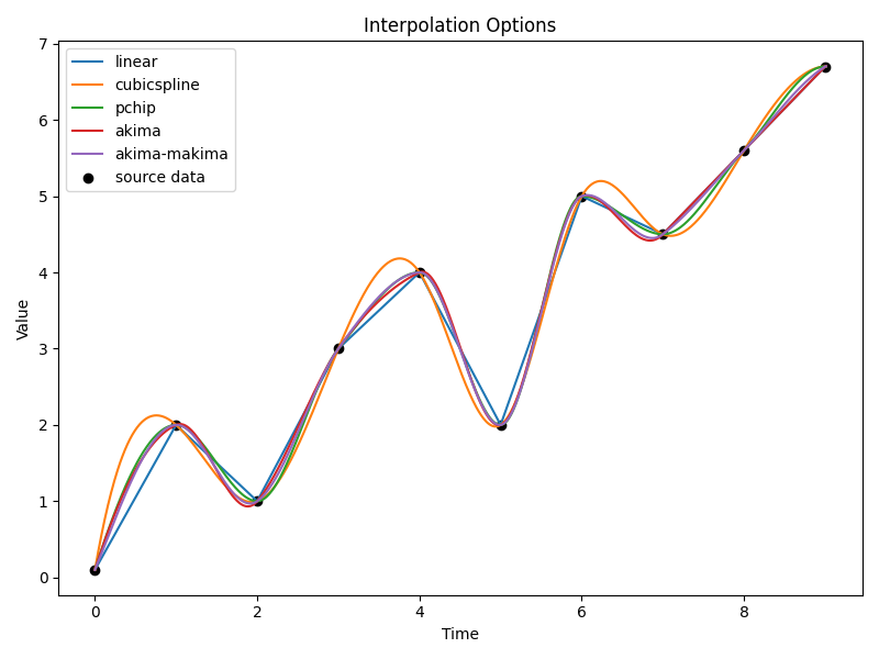
BASE works by estimating the source concentration at each of a prescribed set of inflection points. The source concentration is then interpolated between these points to estimate the source concentration at any time. The interpolation method is defined by the interpolator argument in the BASESolver class. The following interpolation methods are available:
‘linear’: Linear interpolation between the inflection points.
‘spline’: Spline interpolation between the inflection points.
‘pchip’: Piecewise cubic Hermite interpolating polynomial (PCHIP) interpolation between the inflection points.
‘akima’: Akima spline interpolation between the inflection points.
An example of each of these interpolation outputs is shown below:
Interpolation methods#
A note on priors#
As anyone with experience in Bayesian analysis will know, the choice of prior is critical to the outcome of the analysis. BASE is no different. The prior is the distribution of source concentrations that you believe are possible. This is a subjective choice and should be based on all available information and/or the question you are trying to answer. For example:
if you have no knowledge of the source concentration, you could use a widely spread uniform distribution as your prior.
if you have some estimates of the source concentration, you could define a more informative prior based on this information (e.g. a prior with a mean value of your expected source concentration, and a standard deviation based on your uncertainty in the expected source concentration).
if you want to test whether or not your source concentration is consistent with the observed data, you could use a narrowly defined prior (based on your source concentration) and see if the posterior distribution is consistent with the observed receptor data.
if you want to understand the information the data is providing you can run a “reluctant change prior” The prior distribution is defined such that the source concentration at time t is dependent on the source concentration at time t-1 + a change value. The change value is picked from a normal distribution centered on 0. This means that BASE will preferentially maintain a static concentration unless the observation data requires a change in source concentration.
This is in no way an exhaustive list of possible priors, but it should give you an idea of the types of priors you could use in your analysis and the reasons for choosing them.
Prior schema#
We have implemented a schema for defining priors for BASE. This is loosely based on the schema for pydream (pydream.parameters.SampledParam), but has been modified to capture metadata about the prior distributions to allow result serialisation.
The schema functions as follows:
from komanawa.BASE import BaseSampledParam

BaseSampledParam(distribution, *args, **kwargs)
where:
distribution is an object to define the distribution (e.g. scipy.stats.norm, scipy.stats.uniform, komanawa.BASE.generators.NormalPathGenerator, etc.)
*args and **kwargs are the arguments to pass to the distribution object to define the distribution.
The BaseSampledParam object has the following methods:
serialize(): This method produces a unique string representation of the prior distribution. This is used to store the prior distribution in the results file.
to_pydream_SampledParam(): This method converts the BaseSampledParam object to a pydream.parameters.SampledParam object.
Both of these methods are used internally by BASESolver.run_base() and should not need to be called by the user.
Provided prior support#
We have provided a few classes to help you define your prior distribution. These are:
UniformPathGenerator: This class generates a path of uniform prior distribution based on a minimum and maximum values at each time step. Note this prior does not constrain the model with regards to auto-correlation between time steps, which can create unrealistic source concentration paths.
PsuedoUniformPathGenerator: This class generates a path by picking a start value from a uniform distribution and then picking change changes from a distribution that is made of a uniform distribution and two half normal distributions. This is a more realistic prior than the UniformPathGenerator as it constrains the model to have a more realistic auto-correlation between time steps.
NormalPathGenerator: This class generates a path by picking a start value from a uniform distribution and then picking change changes from a normal distribution. Thus the prior value at time t+1 = value at t + the sampled change.
Note that these classes also have plotting methods to help you visualise the prior distribution.
Technical note on priors (scipy)#
pydream and thus BASE use the scipy.stats distributions to define the prior distributions. This means that you can use any of the distributions provided by scipy.stats to define your prior. Just note that some distributions are not intuitive with their args and kwargs. For example, the uniform distribution is defined as scipy.stats.uniform(loc, scale) where loc is the minimum value and scale is the range of the distribution. This is different to the numpy uniform distribution which is defined as numpy.random.uniform(low, high, size). scipy.stats.uniform(1,2) yields the uniform distribution between 1 and 3, while numpy.random.uniform(1,2) yields the uniform distribution between 1 and 2. Just be sure to check the scipy documentation for the distribution you want to use.
Objective Functions#
By default BASE uses one of two log-likelihood functions to compare the observed data to the modelled data, the function used is defined by whether or not sigma is provided to the BASESolver init.
The first is defined in the BASESolver.log_likelihood_no_sigma() method. This is defined as:
where:
\(C_{\text{obs},i}\) is the observed concentration at time i
\(C_{\text{mod},i}\) is the modelled concentration at time i
\(n\) is the number of observations
We chose this log-likelihood function as it is a common way to compare observed data to modelled data without any knowledge of \(\sigma_{\text{obs},i}\) (the uncertainty in the observed data). \(\sigma_{\text{obs},i}\) typically encompasses both the measurement error (e.g. from the lab) and error based on the model structure (e.g. predicting annual source concentrations, which excludes other factors like recharge spikes and seasonal variations).
The second is defined in the BASESolver.log_likelihood_sigma() method. This is defined as:
where:
\(C_{\text{obs},i}\) is the observed concentration at time i
\(C_{\text{mod},i}\) is the modelled concentration at time i
\(n\) is the number of observations
\(\sigma_i\) is the uncertainty in the observed concentration at time i
However, you can define you own objective function as you see fit. To do this you need to create a subclass of the BASESolver class and overwrite the log_likelihood() method. This method should return the log-likelihood of the modelled data given the observed data. The method signature is: log_likelihood(self, params). For example you could define a log-likelihood function based on the absolute residuals (rather than the relative residuals) as follows:
from komanawa.BASE import BASESolver

class MyBASESolver(BASESolver):
    def log_likelihood_no_sigma(self, params):

        modelled = self._predict(*params)
        true = self.ts_data.values
        deltas = (true - modelled)
        likelihood = -len(self.t) / 2 * np.log((deltas ** 2).sum())
        return log_likelihood

solver = MyBASESolver(...)
solver.run_base(...)
Note that the Dreams method expects to maximise the log-likelihood function, so you should ensure that your log-likelihood function is defined such that a higher value is a better fit to the data.